45 how to add total labels to stacked column chart in excel

100% Stacked Area Chart in Excel - Excel Unlocked To do that, you need to add the data labels on the chart:- Select the chart. Click on the + button on the top right corner of the chart Mark the data labels from there Now after adding the Data Labels, you can see both the percentage contributions and their values. You can learn more about adding and deleting chart elements from here. Solved: Getting a Target Line on a Stacked Bar Chart - Power BI Getting a Target Line on a Stacked Bar Chart. 02-25-2022 07:11 AM. I have a request to show a target line on a stacked bar chart visual. I need a target for each of these six bars as drawn in blue below. I added a measure as a constant line, but that gives me the sum of all six targets and not a unique value for each bar.

How to add Data label in Stacked column chart of Pivot charts Hello friends, I'm tring to make a Pivot chart with stacked column graph. In where, i couldn't add data label for cumulative sum of value in Data label. Where i could only add data label to individual stacks in column graph. It found possible with normal stacked column chart without pivot...

How to add total labels to stacked column chart in excel

How to ☝️ Create a Stacked Waterfall Chart in Excel Highlight all data in your chart ( A1:D7 ). 2. Go to the Insert tab. 3. Choose Insert Column or Bar Chart from the Chart menu. 4. Pick Stacked Column. Just like that, you've got your chart! 5. Right-click on the Baseline section of the columns ( blue ). 6. Pick Format Data Series. 7. Choose the Fill & Line option. 8. Select No fill and No line. Sparklines and data bars in a paginated report - Microsoft Report ... You cannot add a sparkline to a detail group in a table. Because sparklines display aggregated data, they must go in a cell associated with a group. Sparklines and data bars have the same basic chart elements of categories, series, and values, but they have no legend, axis lines, labels, or tick marks. How to Show Percentages in Stacked Column Chart in Excel? Follow the below steps to show percentages in stacked column chart In Excel: Step 1: Open excel and create a data table as below. Step 2: Select the entire data table. Step 3: To create a column chart in excel for your data table. Go to "Insert" >> "Column or Bar Chart" >> Select Stacked Column Chart. Step 4: Add Data labels to the chart.

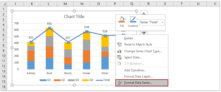
How to add total labels to stacked column chart in excel. How to Create a Cumulative Sum Chart in Excel (With Example) Step 3: Create Bar Chart with Average Line. Next, highlight the cell range A1:C13, then click the Insert tab along the top ribbon, then click Clustered Column within the Charts group. Next, right click anywhere on the chart and then click Change Chart Type: In the new window that appears, click Combo and then click OK: How to Add Total Values to Stacked Bar Chart in Excel Step 4: Add Total Values. Next, right click on the yellow line and click Add Data Labels. Next, double click on any of the labels. In the new panel that appears, check the button next to Above for the Label Position: Next, double click on the yellow line in the chart. In the new panel that appears, check the button next to No line: How to Add Total Values to Stacked Bar Chart in Excel In the new window that appears, click Combo and then choose Stacked Column for each of the products and choose Line for the Total, then click OK: The following chart will be created: Step 4: Add Total Values. Next, right click on the yellow line and click Add Data Labels. The following labels will appear: Next, double click on any of the labels. How to Hack Excel — and Add Totals to the Tops of Stacked Column Charts Edit the chart type and choose the Grand Total series to be something other than a stacked column. Same result, one more step, but a step that can keep the chart looking this way even if the data changes and your axis needs to change as well. Gimme More…

Ordering the stacked column from smallest to the l ... - Power BI Ordering the stacked column from smallest to the largest. 09-28-2021 11:58 PM. Hi, I checked if this question has been asked before but couldn't find a similar one. So I have a chart like below. Its similar to the total number of items sold through different websites. The stacked chart is picking up name of the websites in asceding order and I ... 3 Ways to Create Excel Clustered Stacked Column Charts Create a pivot table, with fields for the chart's horizontal axis in the Row area. Put field that you want to "stack" in the Column area. Then, create a Stacked Column chart from the pivot table. Set the gap width to about 20%, to make the columns wider. Multiple Stacked Columns - Microsoft Community >Basically you need the data, and insert a Chart of columns, according to the print. And then you can adjust the layout options according to your needs, using the color and formatting options. Answer here so I can continue helping you. How do you label data points in Excel? - profitclaims.com Right click the data series in the chart, and select Add Data Labels > Add Data Labels from the context menu to add data labels. 2. Click any data label to select all data labels, and then click the specified data label to select it only in the chart. 3.

How to Add Stacked Bar Totals in Google Sheets or Excel Add another series for the total (calculated), making sure it displays in the chart Change the chart type to Show data labels, and align them so they're at the bottom of the bar. Change the colour of the bar to transparent. Adjust the axis More details — step by step stacked bar totals You can access a workbook with this chart in it here. Label line chart series - Get Digital Help To label each line we need a cell range with the same size as the chart source data. Simply copy the chart source data range and paste it to your worksheet, then delete all data. All cells are now empty. Copy categories (Regions in this example) and paste to the last column (2018). Those correspond to the last data points in each series. 100% Stacked Column Chart in Excel - Inserting, Usage, Reading Go to Insert Tab. In the Charts group, click on column chart button. Select the 100% Stacked Column Chart from the 2-D Column Chart Section. Reading 100% Stacked Column Chart The chart inserted in the above section would be:- Excel has an inbuilt algorithm that decides the orientation of rows and columns in the chart. excel - How to add Data label in Stacked column chart of Pivot charts ... I'm tring to make a Pivot chart with stacked column graph. In where, i couldn't add data label for cumulative sum of value in Data label. Where i could only add data label to individual stacks in column graph. It found possible with normal stacked column chart without pivot chart.

How to Create Stacked Bar Chart with Line in Excel (2 Suitable Examples) Steps. At first, select the range of cells B6 to E12. Then, go to the Insert tab in the ribbon. After that, from the Charts group, select Recommended Charts option. The Insert Chart dialog box will appear. From there, select the Stacked Bar chart. Finally, click on OK.

How to add percentage to bar chart in Excel - profitclaims.com To build a chart from this data, we need to select it. Then, in the Insert menu tab, under the Charts section, choose the Stacked Column option from the Column chart button. Your first results might not be exactly what you expect. In this example, Excel chose the Regions as the X-Axis and the Years as the Series data.

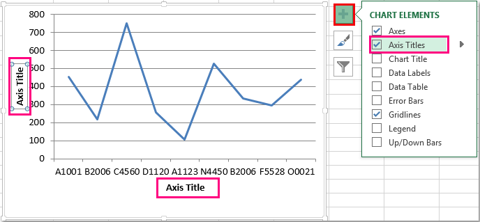
How to Add Axis Titles in a Microsoft Excel Chart Click the Add Chart Element drop-down arrow and move your cursor to Axis Titles. In the pop-out menu, select "Primary Horizontal," "Primary Vertical," or both. If you're using Excel on Windows, you can also use the Chart Elements icon on the right of the chart. Check the box for Axis Titles, click the arrow to the right, then check ...

Stacked Column Chart Data Label Format | Dashboards & Charts | Excel ... February 4, 2022 - 1:45 am. I am having a problem with the format of data labels for a stacked column chart. Having formatted the data labels to my liking, if another series added then the label format of the new series reverts to the default. Custom formatting does not persist when there is dynamic data. I can create a Chart Template but not a ...

How to Make a 100% Stacked Column Chart in Excel To add data labels on the stacked columns, Click on the plus icon at the top-right corner of the chart. In the Chart Elements, go to Data Labels. Now you will see different positioning options such as, Center Inside End Inside Base Data Callout You can select any of them as per your requirement, but I'm selecting Center here.

Position labels in a paginated report chart - Microsoft Report Builder ... To change the position of point labels in an Area, Column, Line or Scatter chart. Create an Area, Column, Line or Scatter chart. On the design surface, right-click the chart and select Show Data Labels. Open the Properties pane. On the View tab, click Properties. On the design surface, click the series.

How to Apply a Filter to a Chart in Microsoft Excel Go to the Home tab, click the Sort & Filter drop-down arrow in the ribbon, and choose "Filter.". Click the arrow at the top of the column for the chart data you want to filter. Use the Filter section of the pop-up box to filter by color, condition, or value. When you finish, click "Apply Filter" or check the box for Auto Apply to see ...

Stacked Bar Chart Matplotlib - Complete Tutorial - Python Guides Let's see an example where we create a stacked bar chart using pandas dataframe: In the above example, we import matplotlib.pyplot, numpy, and pandas library. After this, we create data by using the DataFrame () method of the pandas. Then, print the DataFrame and plot the stacked bar chart by using the plot () method.

Share :