39 pivot table 2 row labels

Excel Pivot Table Row labels - Stack Overflow 1 Answer. Right click on the pivot, go to PivotTable Options, Display Tab. Click on "Classic Pivot Table Layout". Go to each field (column), right click, field settings, layout & print tab. Click on "Repeat Item Labels". That should give you the table you're looking for. Pivot Table Multiple Row Labels? [SOLVED] - excelforum.com You can, of course, create a pivot table that sums the values just at the owner level. then, create a second pivot table that sums the values at the Engineer level. If you need to present this data in a contiguous table, you can create a new Excel table and reference to the pivot table values with formulas (=PivotTableSheet!A1) cheers

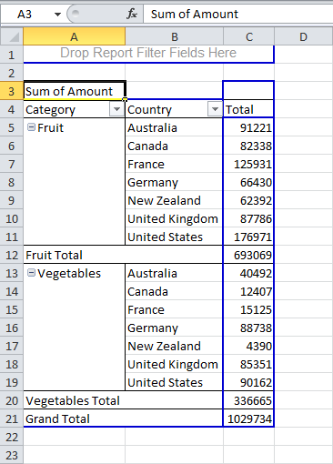
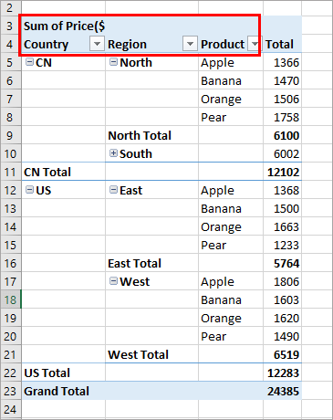
Multi-level Pivot Table in Excel (In Easy Steps) - Excel Easy First, insert a pivot table. Next, drag the following fields to the different areas. 1. Category field and Country field to the Rows area. 2. Amount field to the Values area. Below you can find the multi-level pivot table. Multiple Value Fields First, insert a pivot table. Next, drag the following fields to the different areas. 1.

Pivot table 2 row labels

Automatic Row And Column Pivot Table Labels - How To Excel At Excel Select the data set you want to use for your table The first thing to do is put your cursor somewhere in your data list Select the Insert Tab Hit Pivot Table icon Next select Pivot Table option Select a table or range option Select to put your Table on a New Worksheet or on the current one, for this tutorial select the first option Click Ok Remove PivotTable Duplicate Row Labels [SOLVED] Re: Remove PivotTable Duplicate Row Labels Sometimes when the cells are stored in different formats within the same column in the raw data, they get duplicated. Also, if there is space/s at the beginning or at the end of these fields, when you filter them out they look the same, however, when you plot a Pivot Table, they appear as separate headers. Excel Pivot Table with nested rows | Basic Excel Tutorial Insert your pivot table. Click Insert Menu, under Tables group choose PivotTable. 2. Once you create your pivot table, add all the fields you need to analyze data. How to add the fields. Select the checkbox on each field name you desire in the field section. The selected fields are added to the Row Labels area in the layout section.

Pivot table 2 row labels. pivot table how to combine 2 row labels | MrExcel Message Board Excel Questions pivot table how to combine 2 row labels sdsurzh Nov 6, 2013 S sdsurzh Board Regular Joined Sep 27, 2009 Messages 248 Nov 6, 2013 #1 Hi, i am having the pivot table in the below format. my concern is how i can combine both A & AA together the source is from data connection and not from the excel. Excel Pivot Table Report - Clear All, Remove Filters, Select … 12. Printing a Pivot Table report, Repeat Row Labels, Set Print Titles, Insert Page Breaks, Print Area, Print Layout. Refer complete Tutorial on working with Pivot Tables using VBA: Create and Customize Pivot Table reports, using vba Pivot Table Options tab - Actions group Customizing a Pivot Table report: When you insert a Pivot Table, a blank Pivot Table report is created in the … How to Create a Pivot Table in Excel: A Step-by-Step Tutorial 31.12.2021 · Step 4. Drag and drop a field into the "Row Labels" area. After you've completed Step 3, Excel will create a blank pivot table for you. Your next step is to drag and drop a field — labeled according to the names of the columns in your spreadsheet — into the Row Labels area. This will determine what unique identifier — blog post title ... Multiple Row Labels In Pivot Table | Brokeasshome.com How To Combine Data From Two Pivot Tables; Can You Have 2 Row Labels In A Pivot Table; Home / Uncategorized / Multiple Row Labels In Pivot Table. Multiple Row Labels In Pivot Table. masuzi 24 mins ago Uncategorized Leave a comment 0 Views.

Multiple row labels on one row in Pivot table - MrExcel Message Board I figured it out - Right click on your pivot table and choose pivot table options/display. Click on "Classic PivotTable layout" Then click on where it is subtotaling your row label and uncheck the subtotal option. D dudeshane0 New Member Joined Oct 23, 2014 Messages 1 Jan 19, 2015 #6 Gerald Higgins said: How to Format Excel Pivot Table - Contextures Excel Tips 22.06.2022 · Video: Change Pivot Table Labels. Watch this short video tutorial to see how to make these changes to the pivot table headings and labels. Get the Sample File. No Macros: To experiment with pivot table styles and formatting, download the sample file. The zipped file is in xlsx format, and and does NOT contain any macros. How to Add Rows to a Pivot Table: 9 Steps (with Pictures) - wikiHow 10.08.2022 · Click the tab that contains the data you're using in your pivot table, and make sure it contains the data you want to use to create your new row. For example, if you want to add a row for a specific purchase, make sure that purchase is … What is a Pivot Table & How to Create It? Complete 2022 Guide One difference is that we no longer have Row Labels. Instead, we have Column Labels. Column Labels still refer to the colors red and black. It is just the fact that they now label each of the columns. As with Row labels, Column Labels are placed at the beginning of the columns and they happen to be one next to each other – thus forming a row.

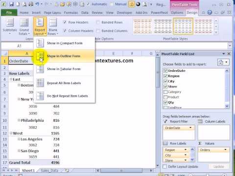
Design the layout and format of a PivotTable Change a PivotTable to compact, outline, or tabular form Change the way item labels are displayed in a layout form Change the field arrangement in a PivotTable Add fields to a PivotTable Copy fields in a PivotTable Rearrange fields in a PivotTable Remove fields from a PivotTable Change the layout of columns, rows, and subtotals Pivot table row labels in separate columns • AuditExcel.co.za Our preference is rather that the pivot tables are shown in tabular form (all columns separated and next to each other). You can do this by changing the report format. So when you click in the Pivot Table and click on the DESIGN tab one of the options is the Report Layout. Click on this and change it to Tabular form. How to Add Two-Tier Row Labels to Pivot Tables in Google Sheets Step 1: Click on any cell in the Pivot Table so that the Pivot table editor sidebar appears on the right side of Google Sheets. Pivot Table, with Pivot table editor sidebar visible. ‍ As you can see, the item column is used as the row labels or headers in the Pivot table. Pivot Table "Row Labels" Header Frustration Pivot Table "Row Labels" Header Frustration. Hi Everyone please help I can't change my headers from Row Labels in a Pivot Table. Using Excel 365. Labels:

Create a Pivot Table in Excel - The Complete Beginners Guide - QuickExcel

Repeat item labels in a PivotTable - support.microsoft.com Right-click the row or column label you want to repeat, and click Field Settings. Click the Layout & Print tab, and check the Repeat item labels box. Make sure Show item labels in tabular form is selected. Notes: When you edit any of the repeated labels, the changes you make are applied to all other cells with the same label.

Chapter-7: Report Layout in Pivot Table - PK: An Excel Expert

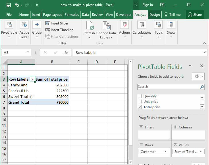
How to Add Rows to a Pivot Table: 9 Steps (with Pictures) - wikiHow 2 Click any cell in the PivotTable. This opens the PivotTable Fields panel on the right side of Excel. If you have already moved the appropriate field to the Rows area but don't see a row that's in your source data, just press Alt + F5 or right-click the pivot table and select Refresh. 3 Drag a field into the "Rows" area on PivotTable Fields.

How to Know the Pivot Field Orientation in Excel Pivot Table with VBA | Microsoft Power BI Kingdom

How to Use Excel Pivot Table Label Filters - Contextures Excel Tips To change the Pivot Table option, and allow multiple filters, follow these steps: Right-click a cell in the pivot table, and click PivotTable Options. In the PivotTable Options dialog box, click the Totals & Filters tab. In the Filters section, add a check mark to 'Allow multiple filters per field.'. Click the OK button, to apply the setting ...

Changing Order of Row Labels in Pivot Table - YouTube

Pivot Table adding "2" to value in answer set 1) Right click your pivot table -> Pivot table options -> Data -> Change "Number of items to retain per field" to NONE 2) Wipe all rows in your data source except for the headers 3) Refresh the pivot table 4) Save, and close all instances of Excel 5) Reopen the file, and paste your data 6) Refresh the pivot table

Repeat Headings in Excel 2010 Pivot Table - YouTube

How to Create Excel Pivot Table (Includes practice file) 28.06.2022 · The area to the left results from your selections from [1] and [2]. You’ll see that the only difference I made in the last pivot table was to drag the AGE GROUP field underneath the PRECINCT field in the Row Labels quadrant. How to Create Excel Pivot Table. There are several ways to build a pivot table. Excel has logic that knows the field ...

Multiple Row Fields

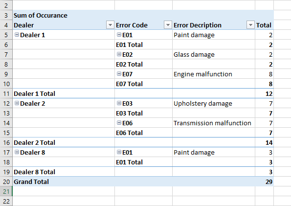
Pivot Table Row Labels In the Same Line - Beat Excel! Then navigate to "Layout & Print" tab and click on "Show item in tabular form" option. Do this procedure also for "Dealer" field and your table will look like this: If you also want dealer names to repeat on each row, reopen "Dealer field settings and check "Repear item labels" option in "Layout & Print" tab.

23 things you should know about Excel pivot tables | Exceljet

Data Labels in Excel Pivot Chart (Detailed Analysis) Add a Pivot Chart from the PivotTable Analyze tab. Then press on the Plus right next to the Chart. Next open Format Data Labels by pressing the More options in the Data Labels. Then on the side panel, click on the Value From Cells. Next, in the dialog box, Select D5:D11, and click OK.

How to reset a custom pivot table row label

Can You Have 2 Row Labels In A Pivot Table | Brokeasshome.com How To Create A Pivot Table With Multiple Row Labels; Can You Combine Two Sets Of Data In A Pivot Table Excel; How Do I Have Multiple Row Labels In A Pivot Table; How To Add More Than One Field In Pivot Table; How To Add More Than One Filter In Pivot Table Google Sheets; How To Combine Data From 2 Pivot Tables; Multiple Row Labels In Pivot Table

How to Use Excel in 2017: 14 Simple Excel Shortcuts, Tips & Tricks

Ranking to a Pivot Table with multiple Row Labels I have a pivot table with multiple Row Labels: Team and Player. I created a second Pts column and used 'Show Values As - Rank Largest to Smallest', but it's not working. It's showing up as '1' for all columns, regardless of whether or not I pick 'Team' or 'Player' as the base field. If I remove 'Team' as a Row Label, however, it works perfectly.

Pivot Table Multiple Row Labels Side By Side | Decorations I Can Make

Pivot table - Wikipedia A pivot table usually consists of row, column and data (or fact) fields.In this case, the column is ship date, the row is region and the data we would like to see is (sum of) units.These fields allow several kinds of aggregations, including: sum, average, standard deviation, count, etc.In this case, the total number of units shipped is displayed here using a sum aggregation.

Pivot table row labels side by side – Excel Tutorials

How to make row labels on same line in pivot table? - ExtendOffice Make row labels on same line with PivotTable Options You can also go to the PivotTable Options dialog box to set an option to finish this operation. 1. Click any one cell in the pivot table, and right click to choose PivotTable Options, see screenshot: 2.

How to make row labels on same line in pivot table?

excel - Custom row labels in PivotTable - Stack Overflow 1. you can give nicknames to the fields that you are checking which populate the pivot table. If you go the pivot table data and right click you can change the value field settings to give a custom name to a row/series but I do not know about individual data points. path: pivot table data => right click => select Field Settings => edit custom name.

Pivot table row labels side by side

Excel Pivot Table Subtotals - Contextures Excel Tips 01.02.2022 · In the pivot table shown below, Service is in the Row Labels area, Lead Tech is in the Column Labels area, and Labor Cost is in the Values area. Because Service is the only field in the Row Labels area, it has no subtotal. Multiple Row Fields. When you add another field to the Row Labels area, a subtotal is automatically created for the first ...

Excel Help: Simple method to make Pivot table

Quick tip: Rename headers in pivot table so they are presentable 15.03.2018 · Change the order of pivot table row labels; First and last date of a sale with pivots; Introduction to pivot tables; Pivots from multiple tables; What is your favorite pivot tip? Please share in comments. Share on facebook. Facebook Share on twitter. Twitter Share on linkedin . LinkedIn Share this tip with your colleagues Get FREE Excel + Power BI Tips. Simple, fun and …

Can I use the union of two columns values in Excel as row labels in a Pivot Table? - Super User

How to add side by side rows in excel pivot table - AnswerTabs To display more pivot table rows side by side, you need to turn on the Classic PivotTable layout and modify Field settings. For example will be used the following table: You have to right-click on pivot table and choose the PivotTable options. Then swich to Display tab and turn on Classic PivotTable layout:

Pivot Table Multiple Row Labels Side By Side | Decorations I Can Make

How to rename group or row labels in Excel PivotTable? - ExtendOffice You can rename a group name in PivotTable as to retype a cell content in Excel. Click at the Group name, then go to the formula bar, type the new name for the group. Rename Row Labels name To rename Row Labels, you need to go to the Active Field textbox. 1. Click at the PivotTable, then click Analyze tab and go to the Active Field textbox. 2.

Share :