39 excel chart show labels
Dynamically Label Excel Chart Series Lines - My Online Training Hub Step 1: Duplicate the Series. The first trick here is that we have 2 series for each region; one for the line and one for the label, as you can see in the table below: Select columns B:J and insert a line chart (do not include column A). To modify the axis so the Year and Month labels are nested; right-click the chart > Select Data > Edit the ... How to Create a Bar Chart With Labels Above Bars in Excel In the chart, right-click the Series "Dummy" Data Labels and then, on the short-cut menu, click Format Data Labels. 15. In the Format Data Labels pane, under Label Options selected, set the Label Position to Inside End. 16. Next, while the labels are still selected, click on Text Options, and then click on the Textbox icon. 17.
How to Add Labels to Show Totals in Stacked Column Charts in Excel The chart should look like this: 8. In the chart, right-click the "Total" series and then, on the shortcut menu, select Add Data Labels. 9. Next, select the labels and then, in the Format Data Labels pane, under Label Options, set the Label Position to Above. 10. While the labels are still selected set their font to Bold. 11.

Excel chart show labels
Add / Move Data Labels in Charts - Excel & Google Sheets Add and Move Data Labels in Google Sheets. Double Click Chart. Select Customize under Chart Editor. Select Series. 4. Check Data Labels. 5. Select which Position to move the data labels in comparison to the bars. How to hide zero data labels in chart in Excel? - ExtendOffice Sometimes, you may add data labels in chart for making the data value more clearly and directly in Excel. But in some cases, there are zero data labels in the chart, and you may want to hide these zero data labels. Here I will tell you a quick way to hide the zero data labels in Excel at once. Hide zero data labels in chart Chart Labels | MrExcel Message Board 29 minutes ago. #1. I have a chart that has 2 series (Budget - The green column & Spend - The blue column) where I want to hide labels where there is a zero value. I also need to show the label to 1 decimal place of the unit type (thousands) but where I have applied the number format of '#""' to the Spend column, it shows with no decimal places.
Excel chart show labels. How to display text labels in the X-axis of scatter chart in Excel? Actually, there is no way that can display text labels in the X-axis of scatter chart in Excel, but we can create a line chart and make it look like a scatter chart. 1. Select the data you use, and click Insert > Insert Line & Area Chart > Line with Markers to select a line chart. See screenshot: 2. How to add axis label to chart in Excel? - ExtendOffice You can insert the horizontal axis label by clicking Primary Horizontal Axis Title under the Axis Title drop down, then click Title Below Axis, and a text box will appear at the bottom of the chart, then you can edit and input your title as following screenshots shown. 4. How To Add Axis Labels In Excel [Step-By-Step Tutorial] First off, you have to click the chart and click the plus (+) icon on the upper-right side. Then, check the tickbox for 'Axis Titles'. If you would only like to add a title/label for one axis (horizontal or vertical), click the right arrow beside 'Axis Titles' and select which axis you would like to add a title/label. Editing the Axis Titles Excel charts: add title, customize chart axis, legend and data labels Click anywhere within your Excel chart, then click the Chart Elements button and check the Axis Titles box. If you want to display the title only for one axis, either horizontal or vertical, click the arrow next to Axis Titles and clear one of the boxes: Click the axis title box on the chart, and type the text.
Edit titles or data labels in a chart - support.microsoft.com On a chart, click the label that you want to link to a corresponding worksheet cell. On the worksheet, click in the formula bar, and then type an equal sign (=). Select the worksheet cell that contains the data or text that you want to display in your chart. You can also type the reference to the worksheet cell in the formula bar. Add or remove data labels in a chart - support.microsoft.com Click the data series or chart. To label one data point, after clicking the series, click that data point. In the upper right corner, next to the chart, click Add Chart Element > Data Labels. To change the location, click the arrow, and choose an option. If you want to show your data label inside a text bubble shape, click Data Callout. How to Insert Axis Labels In An Excel Chart | Excelchat We will again click on the chart to turn on the Chart Design tab We will go to Chart Design and select Add Chart Element Figure 6 - Insert axis labels in Excel In the drop-down menu, we will click on Axis Titles, and subsequently, select Primary vertical Figure 7 - Edit vertical axis labels in Excel Excel charts: how to move data labels to legend You can't do that, but you can show a data table below the chart instead of data labels: Click anywhere on the chart. On the Design tab of the ribbon (under Chart Tools), in the Chart Layouts group, click Add Chart Element > Data Table > With Legend Keys (or No Legend Keys if you prefer)
Change the format of data labels in a chart To get there, after adding your data labels, select the data label to format, and then click Chart Elements > Data Labels > More Options. To go to the appropriate area, click one of the four icons ( Fill & Line, Effects, Size & Properties ( Layout & Properties in Outlook or Word), or Label Options) shown here. How to Use Cell Values for Excel Chart Labels Select the chart, choose the "Chart Elements" option, click the "Data Labels" arrow, and then "More Options." Uncheck the "Value" box and check the "Value From Cells" box. Select cells C2:C6 to use for the data label range and then click the "OK" button. The values from these cells are now used for the chart data labels. Display every "n" th data label in graphs - Microsoft Community you can use a free tool created by Rob Bovey, called the XY Chart Labeler. With this tool you can assign a range of cells to be the labels for chart series, instead of the Excel defaults. Using a formula, you can have a text show up in every nth cell and then use that range with the XY Chart Labeler to display as the series label. How to format axis labels as thousands/millions in Excel? Right click at the axis you want to format its labels as thousands/millions, select Format Axisin the context menu. 2. In the Format Axisdialog/pane, click Number tab, then in theCategorylist box, select Custom, and type[>999999] #,,"M";#,"K"into Format Codetext box, and click Addbutton to add it toTypelist. See screenshot: 3.
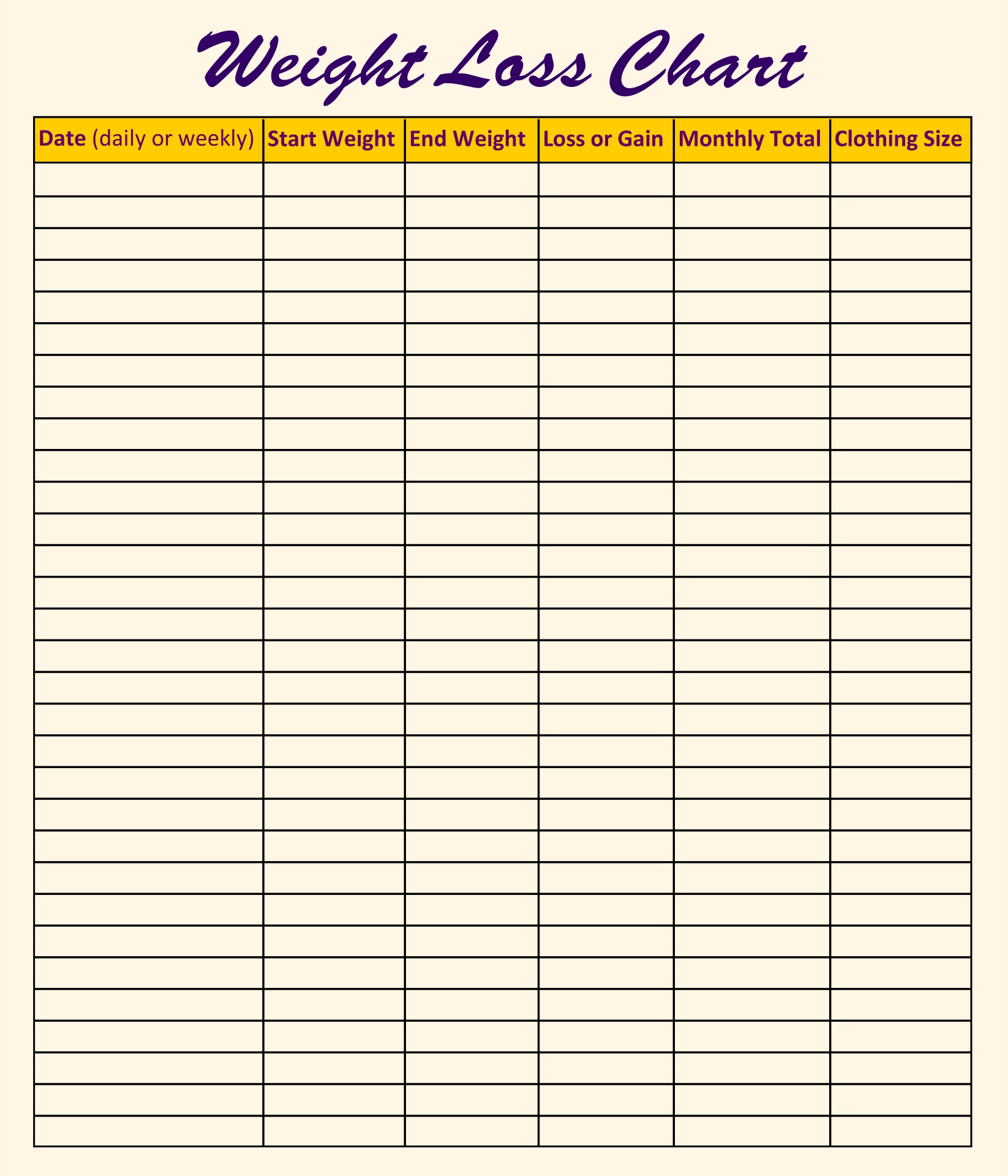
8 Best Images of Weight Loss Charts Printable Monthly - Free Printable Weight Loss Chart, Weight ...
Show or hide a chart legend or data table Select a chart and then select the plus sign to the top right. Point to Legend and select the arrow next to it. Choose where you want the legend to appear in your chart. Hide a chart legend Select a legend to hide. Press Delete. Show or hide a data table Select a chart and then select the plus sign to the top right.
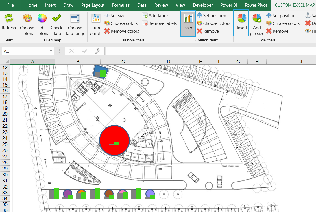
Create your custom filled map (choropleth map) for regions, warehouse, factory, process etc ...
How to Create a Bar Chart With Labels Inside Bars in Excel In the chart, right-click the Series "# Footballers" Data Labels and then, on the short-cut menu, click Format Data Labels. 8. In the Format Data Labels pane, under Label Options selected, set the Label Position to Inside End. 9. Next, in the chart, select the Series 2 Data Labels and then set the Label Position to Inside Base. 10.
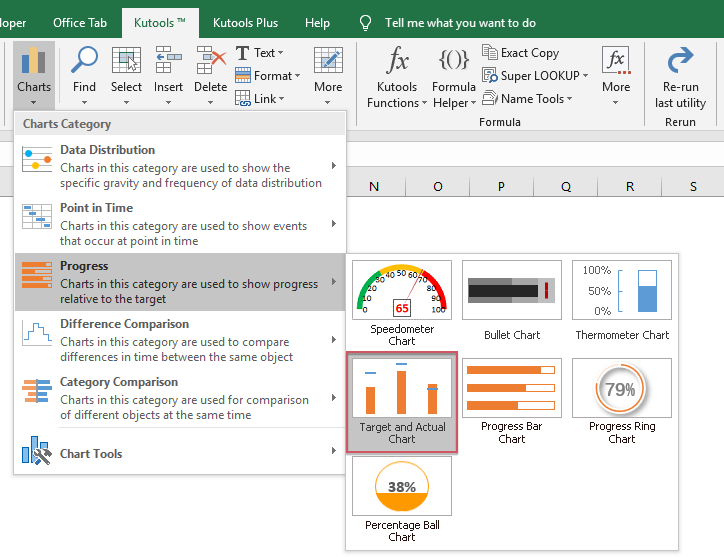
Quickly Create An Actual Vs Target Chart In Excel
Excel tutorial: How to use data labels Generally, the easiest way to show data labels to use the chart elements menu. When you check the box, you'll see data labels appear in the chart. If you have more than one data series, you can select a series first, then turn on data labels for that series only. You can even select a single bar, and show just one data label.
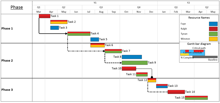
Project Critical Path in a Report | OnePager Pro
How to Add Labels to Scatterplot Points in Excel - Statology Next, click anywhere on the chart until a green plus (+) sign appears in the top right corner. Then click Data Labels, then click More Options… In the Format Data Labels window that appears on the right of the screen, uncheck the box next to Y Value and check the box next to Value From Cells.

Waterfall Chart in Excel - Easiest method to build.
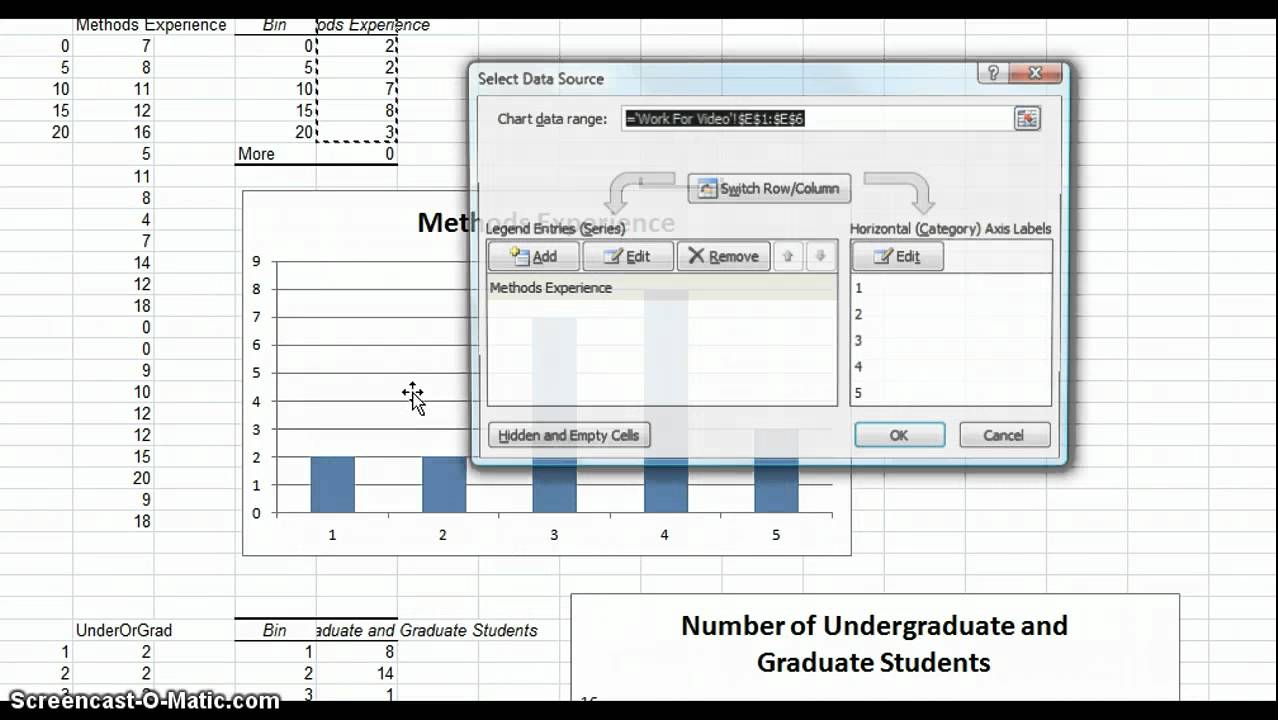
Change axis labels in a chart - support.microsoft.com Right-click the category labels you want to change, and click Select Data. In the Horizontal (Category) Axis Labels box, click Edit. In the Axis label range box, enter the labels you want to use, separated by commas. For example, type Quarter 1,Quarter 2,Quarter 3,Quarter 4. Change the format of text and numbers in labels
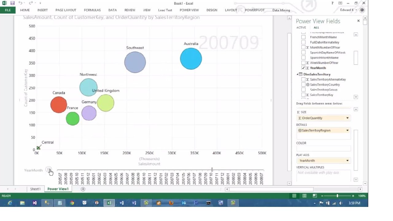
Excel 2013 PowerView Animated Scatterplot/Bubble Chart Business Intelligence Tutorial - YouTube
How to add or move data labels in Excel chart? - ExtendOffice In Excel 2013 or 2016. 1. Click the chart to show the Chart Elements button . 2. Then click the Chart Elements, and check Data Labels, then you can click the arrow to choose an option about the data labels in the sub menu. See screenshot: In Excel 2010 or 2007. 1. click on the chart to show the Layout tab in the Chart Tools group. See ...
Changing X-Axis Values - YouTube
Data labels not displaying when chart is pasted into PowerPoint When I paste an Excel chart to PowerPoint (2013), some people do not see the data labels strings, just the " [cell range]", as Scott reported. In my PowerPoint, the labels display just fine. My colleague, who sees these [cell range] labels, has PowerPoint 2010. I found out that the problem happens also if I create the chart in PowerPoint from ...

How to Add Data Labels to your Excel Chart in Excel 2013 - YouTube
charts - Excel, giving data labels to only the top/bottom X% values ... Here is what you can do, in stages: 1) Create a data set next to your original series column with only the values you want labels for (again, this can be formula driven to only select the top / bottom n values). See column D below. 2) Add this data series to the chart and show the data labels. 3) Set the line color to No Line, so that it does ...
Post a Comment for "39 excel chart show labels"