40 excel column chart labels
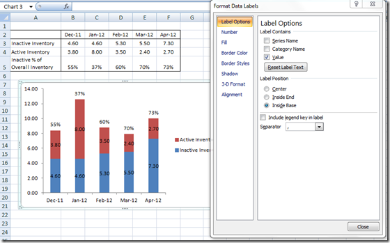
100% Stacked Column Chart labels - Microsoft Community Select the data on the data sheet, then right-click on the selection and choose Format Cells. In the Format Cells dialog, choose the Number tab and set the Category to Percentage. OK out. The data labels show the percentage value of the data. Or click on the data labels in a series and choose Format Data Labels. The Format Data Labels pane opens. how to align x-axis labels in column chart? - MrExcel Message Board The Excel help page "Change the display of chart axes" ( click here) [1] explains: "You can also change the horizontal alignment of axis labels, by right-clicking the axis, and then click Align Left Button image, Center Button image, or Align Right Button image on the Mini toolbar." When I do that with labels at -45 deg as above, I see very ...
Change the format of data labels in a chart To get there, after adding your data labels, select the data label to format, and then click Chart Elements > Data Labels > More Options. To go to the appropriate area, click one of the four icons ( Fill & Line, Effects, Size & Properties ( Layout & Properties in Outlook or Word), or Label Options) shown here.

Excel column chart labels
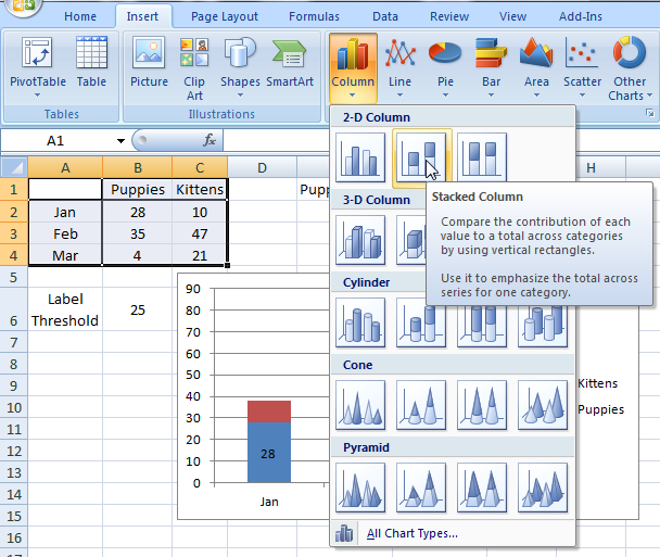
How to wrap X axis labels in a chart in Excel? - ExtendOffice 1. Double click a label cell, and put the cursor at the place where you will break the label. 2. Add a hard return or carriages with pressing the Alt + Enter keys simultaneously. 3. Add hard returns to other label cells which you want the labels wrapped in the chart axis. Then you will see labels are wrapped automatically in the chart axis. How to I rotate data labels on a column chart so that they are ... To change the text direction, first of all, please double click on the data label and make sure the data are selected (with a box surrounded like following image). Then on your right panel, the Format Data Labels panel should be opened. Go to Text Options > Text Box > Text direction > Rotate How to Use Cell Values for Excel Chart Labels Select range A1:B6 and click Insert > Insert Column or Bar Chart > Clustered Column. The column chart will appear. We want to add data labels to show the change in value for each product compared to last month. Select the chart, choose the "Chart Elements" option, click the "Data Labels" arrow, and then "More Options."
Excel column chart labels. How to create Custom Data Labels in Excel Charts Create a simple line chart while selecting the first two columns only. Now Add Regular Data Labels. Two ways to do it. Click on the Plus sign next to the chart and choose the Data Labels option. We do NOT want the data to be shown. To customize it, click on the arrow next to Data Labels and choose More Options … How to add data labels from different column in an Excel chart? Right click the data series in the chart, and select Add Data Labels > Add Data Labels from the context menu to add data labels. 2. Click any data label to select all data labels, and then click the specified data label to select it only in the chart. 3. Stagger long axis labels and make one label stand out in an Excel ... This is hard for the viewer to read. The common approach to solving this issue is to add a New Line character at the start of every second axis label by pressing Alt+Enter at the start of the label text or by using a formula to add CHAR(10) [the New Line character] at the start of the text (described well by Excel MVP Jon Peltier here).The method also involves forcing Excel to use every label ... Change axis labels in a chart - support.microsoft.com Right-click the category labels you want to change, and click Select Data. In the Horizontal (Category) Axis Labels box, click Edit. In the Axis label range box, enter the labels you want to use, separated by commas. For example, type Quarter 1,Quarter 2,Quarter 3,Quarter 4. Change the format of text and numbers in labels
Change axis labels in a chart in Office - support.microsoft.com The chart uses text from your source data for axis labels. To change the label, you can change the text in the source data. If you don't want to change the text of the source data, you can create label text just for the chart you're working on. In addition to changing the text of labels, you can also change their appearance by adjusting formats. Edit titles or data labels in a chart - support.microsoft.com On a chart, click the label that you want to link to a corresponding worksheet cell. On the worksheet, click in the formula bar, and then type an equal sign (=). Select the worksheet cell that contains the data or text that you want to display in your chart. You can also type the reference to the worksheet cell in the formula bar. Excel tutorial: How to customize axis labels Instead you'll need to open up the Select Data window. Here you'll see the horizontal axis labels listed on the right. Click the edit button to access the label range. It's not obvious, but you can type arbitrary labels separated with commas in this field. So I can just enter A through F. When I click OK, the chart is updated. Chart label in round figures | MrExcel Message Board Apr 29, 2018. #2. If you have chosen the "Add Values From Cell" feature then the format should follow that of the linked cells so you can just format those the way you want or you can select the labels and edit the number format in the chart formatting wizard. in any case, you do not need to label each data point in your series, try to label ...
How to Customize Your Excel Pivot Chart Data Labels - dummies The Data Labels command on the Design tab's Add Chart Element menu in Excel allows you to label data markers with values from your pivot table. When you click the command button, Excel displays a menu with commands corresponding to locations for the data labels: None, Center, Left, Right, Above, and Below. Column Chart with Category Axis Labels Between Columns Click the menu key (between the right Alt and Ctrl buttons on most Windows keyboards) or hold Shift and click the F10 function key to pop up the context menu. Click Change Series Chart Type, and choose XY Scatter. This adds a set of markers along the bottom of the chart (I used blue circles in the chart below) and it adds secondary X and Y axes. How to add total labels to stacked column chart in Excel? Select the source data, and click Insert > Insert Column or Bar Chart > Stacked Column. 2. Select the stacked column chart, and click Kutools > Charts > Chart Tools > Add Sum Labels to Chart. Then all total labels are added to every data point in the stacked column chart immediately. Create a stacked column chart with total labels in Excel Create a multi-level category chart in Excel - ExtendOffice Select the dots, click the Chart Elements button, and then check the Data Labels box. 23. Right click the data labels and select Format Data Labels from the right-clicking menu. 24. In the Format Data Labels pane, please do as follows. 24.1) Check the Value From Cells box;
Do My Excel Blog: How to design a multiple clustered bar chart series in Excel
Excel Custom Chart Labels • My Online Training Hub Custom Excel Chart Label Positions using a dummy or ghost series to force the label position neatly above the columns of data Lookup Pictures in Excel Lookup Pictures in Excel using values in cells returned by data validation lists (drop down lists) or Slicers. No VBA/Macros required!
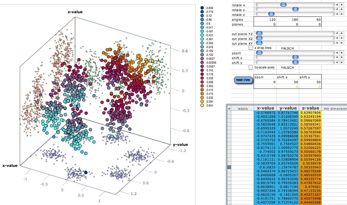
3d scatter plot for MS Excel
Excel charts: add title, customize chart axis, legend and data labels ... Click anywhere within your Excel chart, then click the Chart Elements button and check the Axis Titles box. If you want to display the title only for one axis, either horizontal or vertical, click the arrow next to Axis Titles and clear one of the boxes: Click the axis title box on the chart, and type the text.
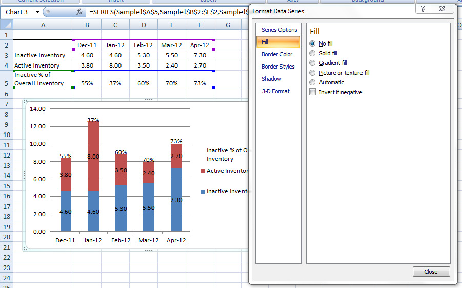
How-to Put Percentage Labels on Top of a Stacked Column Chart - Excel Dashboard Templates
How to Create a Bar Chart With Labels Above Bars in Excel In the Format Data Labels pane, under Label Options selected, set the Label Position to Inside End. 16. Next, while the labels are still selected, click on Text Options, and then click on the Textbox icon. 17. Uncheck the Wrap text in shape option and set all the Margins to zero. The chart should look like this: 18.
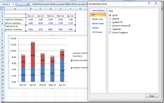
Excel Dashboard Templates How-to Put Percentage Labels on Top of a Stacked Column Chart - Excel ...
How to group (two-level) axis labels in a chart in Excel? Select the source data, and then click the Insert Column Chart (or Column) > Column on the Insert tab. Now the new created column chart has a two-level X axis, and in the X axis date labels are grouped by fruits. See below screen shot: Group (two-level) axis labels with Pivot Chart in Excel

Labeling a Stacked Column Chart in Excel | PolicyViz
How to Add Labels to Show Totals in Stacked Column Charts in Excel The chart should look like this: 8. In the chart, right-click the "Total" series and then, on the shortcut menu, select Add Data Labels. 9. Next, select the labels and then, in the Format Data Labels pane, under Label Options, set the Label Position to Above. 10. While the labels are still selected set their font to Bold. 11.

Excel-User.com: Excel Charts - Add totals labels to Stacked Column chart
How to Insert Axis Labels In An Excel Chart | Excelchat Figure 2 - Adding Excel axis labels. Next, we will click on the chart to turn on the Chart Design tab. We will go to Chart Design and select Add Chart Element. Figure 3 - How to label axes in Excel. In the drop-down menu, we will click on Axis Titles, and subsequently, select Primary Horizontal. Figure 4 - How to add excel horizontal axis ...

3d scatter plot for MS Excel
Adding Labels to Column Charts | Online Excel Training | Kubicle To add data labels, just right-click on a data series and click add data labels. To see the data labels clearly, I'll need to select them and change their color to white. The data labels are determined by the vertical axis of your chart. Currently, the vertical axis shows millions, therefore, my data labels are shown in millions as well.
10 ways to present variance analysis reports in Excel - PakAccountants.com
Add / Move Data Labels in Charts - Excel & Google Sheets Double Click Chart Select Customize under Chart Editor Select Series 4. Check Data Labels 5. Select which Position to move the data labels in comparison to the bars. Final Graph with Google Sheets After moving the dataset to the center, you can see the final graph has the data labels where we want.
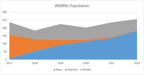
Area Chart in Excel - Easy Excel Tutorial
Text Labels on a Vertical Column Chart in Excel - Peltier Tech Right click on the new series, choose "Change Chart Type" ("Chart Type" in 2003), and select the clustered bar style. There are no Rating labels because there is no secondary vertical axis, so we have to add this axis by hand. On the Excel 2007 Chart Tools > Layout tab, click Axes, then Secondary Horizontal Axis, then Show Left to Right Axis.

microsoft excel - Cannot change column width or add separate data labels in date specific bar ...
How to Make a Column Chart in Excel: A Guide to Doing it Right How to make a column chart in Excel The data shown below was used to create the column chart above. The data is arranged with the labels in the first column and the values in the second column. Nice and simple. The chart will have no problem interpreting this layout. Select the range of cells A2:B6. We have excluded row 1 in our selection.

34 How To Label A Column In Excel - Labels Information List
Add or remove data labels in a chart - support.microsoft.com Click the data series or chart. To label one data point, after clicking the series, click that data point. In the upper right corner, next to the chart, click Add Chart Element > Data Labels. To change the location, click the arrow, and choose an option. If you want to show your data label inside a text bubble shape, click Data Callout.
35 How To Label Columns In Excel - Label Ideas 2021
How to Use Cell Values for Excel Chart Labels Select range A1:B6 and click Insert > Insert Column or Bar Chart > Clustered Column. The column chart will appear. We want to add data labels to show the change in value for each product compared to last month. Select the chart, choose the "Chart Elements" option, click the "Data Labels" arrow, and then "More Options."
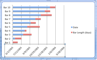
Excel Timelines
How to I rotate data labels on a column chart so that they are ... To change the text direction, first of all, please double click on the data label and make sure the data are selected (with a box surrounded like following image). Then on your right panel, the Format Data Labels panel should be opened. Go to Text Options > Text Box > Text direction > Rotate
Excel Dashboard Templates How-to Make Conditional Label Values in an Excel Stacked Column Chart ...
How to wrap X axis labels in a chart in Excel? - ExtendOffice 1. Double click a label cell, and put the cursor at the place where you will break the label. 2. Add a hard return or carriages with pressing the Alt + Enter keys simultaneously. 3. Add hard returns to other label cells which you want the labels wrapped in the chart axis. Then you will see labels are wrapped automatically in the chart axis.
Excel Dashboard Templates How-to Put Percentage Labels on Top of a Stacked Column Chart - Excel ...
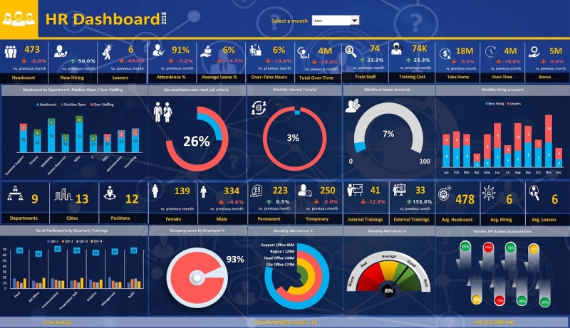
Excel Advanced Dashboard
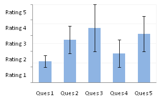
Text Labels on a Vertical Column Chart in Excel - Peltier Tech Blog

How to add total labels to stacked column chart in Excel?
Post a Comment for "40 excel column chart labels"