38 excel graph data labels different series
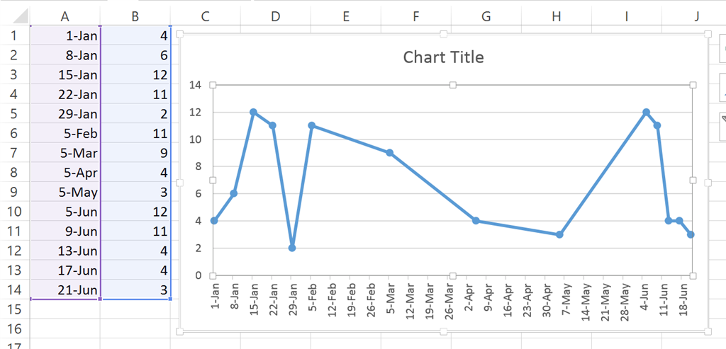
Create Dynamic Chart Data Labels with Slicers - Excel Campus Feb 10, 2016 · Repeat this step for each series in the chart. If you are using Excel 2010 or earlier the chart will look like the following when you open the file. ... This table contains the three options for the different data labels. ... [on the use of Excel]. The problem with the graph is that there is too much detail being presented – we need to show ... How to add data labels from different column in an Excel chart? This method will introduce a solution to add all data labels from a different column in an Excel chart at the same time. Please do as follows: 1. Right click the data series in the chart, and select Add Data Labels > Add Data Labels from the context menu to add data labels. 2. Right click the data series, and select Format Data Labels from the ...
› office-addins-blog › 2018/10/10Find, label and highlight a certain data point in Excel ... Oct 10, 2018 · Add a new data series for the data point. With the source data ready, let's create a data point spotter. For this, we will have to add a new data series to our Excel scatter chart: Right-click any axis in your chart and click Select Data…. In the Select Data Source dialogue box, click the Add button. In the Edit Series window, do the following:
Excel graph data labels different series
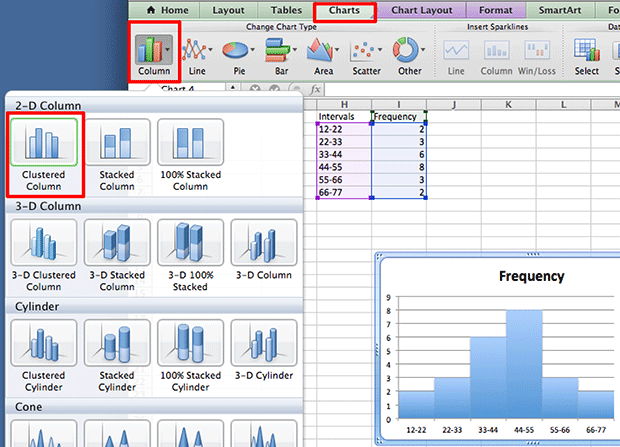
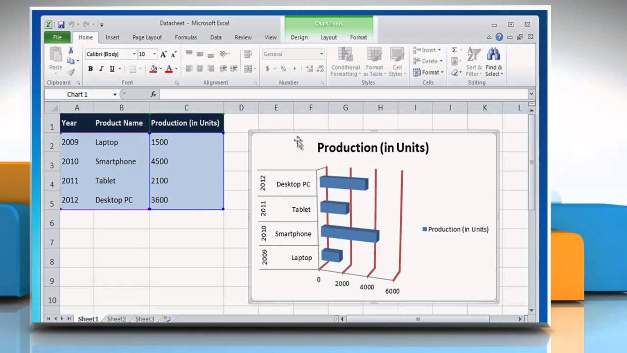
› documents › excelHow to add data labels from different column in an Excel chart? This method will introduce a solution to add all data labels from a different column in an Excel chart at the same time. Please do as follows: 1. Right click the data series in the chart, and select Add Data Labels > Add Data Labels from the context menu to add data labels. 2. Right click the data series, and select Format Data Labels from the ... Excel Charts: Dynamic Label positioning of line series - XelPlus To see the label for the Budget series, perform the following: Select your chart and go to the Format tab, click on the drop-down menu at the upper left-hand portion and select Series "Budget". Go to Layout tab, select Data Labels > Right. Right mouse click on the data label displayed on the chart. Select Format Data Labels. How to create a chart (graph) in Excel and save it as template Oct 22, 2015 · 3. Inset the chart in Excel worksheet. To add the graph on the current sheet, go to the Insert tab > Charts group, and click on a chart type you would like to create.. In Excel 2013 and Excel 2016, you can click the Recommended Charts button to view a gallery of pre-configured graphs that best match the selected data.. In this example, we are creating a 3-D …
Excel graph data labels different series. Dynamically Label Excel Chart Series Lines - My Online Training Hub Step 1: Duplicate the Series. The first trick here is that we have 2 series for each region; one for the line and one for the label, as you can see in the table below: Select columns B:J and insert a line chart (do not include column A). To modify the axis so the Year and Month labels are nested; right-click the chart > Select Data > Edit the ... Custom Data Labels with Colors and Symbols in Excel Charts - [How To] To apply custom format on data labels inside charts via custom number formatting, the data labels must be based on values. You have several options like series name, value from cells, category name. But it has to be values otherwise colors won't appear. Symbols issue is quite beyond me. › Make-a-Bar-Graph-in-ExcelHow to Make a Bar Graph in Excel: 9 Steps (with Pictures) May 02, 2022 · Once you decide on a graph format, you can use the "Design" section near the top of the Excel window to select a different template, change the colors used, or change the graph type entirely. The "Design" window only appears when your graph is selected. Individually Formatted Category Axis Labels - Peltier Tech Format the category axis (vertical axis) to have no labels. Add data labels to the secondary series (the dummy series). Use the Inside Base and Category Names options. Format the value axis (horizontal axis) so its minimum is locked in at zero. You may have to shrink the plot area to widen the margin where the labels appear.
Excel change format 'all data series' bars' of chart This is not possible manually, you have to use a macro. Do as follows: Select one series in the chart. Start the macro recorder. Format the series as you like. Stop the macro recorder. Post the macro here, we can help you to run that on all series in your chart. Important: Do not select anything during the macro recording, just format the series. Changing data label format for all series in a pivot chart To change data labels format, please perform the following steps: Click the pivot chart > + sign near tthe pivot chart > right click data label of any series > Format Data Series... Besides, to move forward, could you please provide the following information? 1. Do all series have data labels when you create a pivot chart? How to group (two-level) axis labels in a chart in Excel? (1) In Excel 2007 and 2010, clicking the PivotTable > PivotChart in the Tables group on the Insert Tab; (2) In Excel 2013, clicking the Pivot Chart > Pivot Chart in the Charts group on the Insert tab. 2. In the opening dialog box, check the Existing worksheet option, and then select a cell in current worksheet, and click the OK button. 3. Edit titles or data labels in a chart - support.microsoft.com The first click selects the data labels for the whole data series, and the second click selects the individual data label. Right-click the data label, and then click Format Data Label or Format Data Labels. Click Label Options if it's not selected, and then select the Reset Label Text check box. Top of Page
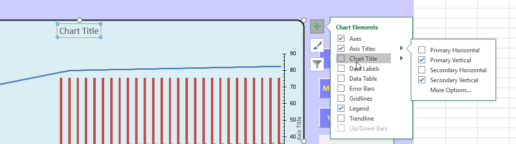
Change the format of data labels in a chart To get there, after adding your data labels, select the data label to format, and then click Chart Elements > Data Labels > More Options. To go to the appropriate area, click one of the four icons ( Fill & Line, Effects, Size & Properties ( Layout & Properties in Outlook or Word), or Label Options) shown here. How to add data labels from different column in an Excel chart? This method will guide you to manually add a data label from a cell of different column at a time in an Excel chart. 1. Right click the data series in the chart, and select Add Data Labels > Add Data Labels from the context menu to add data labels. 2. Click any data label to select all data labels, and then click the specified data label to ... The Excel Chart SERIES Formula - Peltier Tech Data in an Excel chart is governed by the SERIES formula. This formula is only valid in a chart, not in any worksheet cell, but it can be edited just like any other Excel formula. The SERIES Formula. Select a series in a chart. The source data for that series, if it comes from the same worksheet, is highlighted in the worksheet. Change the format of data labels in a chart To get there, after adding your data labels, select the data label to format, and then click Chart Elements > Data Labels > More Options. To go to the appropriate area, click one of the four icons ( Fill & Line, Effects, Size & Properties ( Layout & Properties in Outlook or Word), or Label Options) shown here.
Excel Chart With Time On X Axis - Chart Walls
excel - Change Multiple Chart Series Labels - Stack Overflow Sub UpdateCharts () For Each s In ThisWorkbook.Sheets For Each c In s.ChartObjects c.Activate ActiveChart.FullSeriesCollection (1).Name = s.Name ActiveChart.FullSeriesCollection (2).Name = "=""Trend""" Next Next End Sub Share Improve this answer answered Aug 11, 2015 at 18:08 leal32b 149 8 Hi @leal32b Thanks for the help!
Creating a chart with dynamic labels - Microsoft Excel 2013
How to Create a Graph with Multiple Lines in Excel Click Select Data button on the Design tab to open the Select Data Source dialog box. Select the series you want to edit, then click Edit to open the Edit Series dialog box. Type the new series label in the Series name: textbox, then click OK.

How to Import, Graph, and Label Excel Data in MATLAB: 13 Steps
Dynamically Label Excel Chart Series Lines - My Online Training … Sep 26, 2017 · The Label Series Data contains a formula that only returns the value for the last row of data. You can see in the image below that the formula in cell G5 is: =IF(AND(C6="",C5<>""), [@[UK Data]],NA()) As new data is added the formula dynamically fills down because my data is formatted in an Excel Table , hence the [@[UK Data]] structured ...
:max_bytes(150000):strip_icc()/PieExploded-5be1b86cc9e77c0051098a67.jpg)
Excel Chart Data Series, Data Points, and Data Labels
Change the labels in an Excel data series | TechRepublic Click the Chart Wizard button in the Standard toolbar. Click Next. Click the Series tab. Click the Window Shade button in the Category (X) Axis Labels box. Select B3:D3 to select the labels in your...

Add or remove data labels in a chart - support.microsoft.com Click the data series or chart. To label one data point, after clicking the series, click that data point. In the upper right corner, next to the chart, click Add Chart Element > Data Labels. To change the location, click the arrow, and choose an option. If you want to show your data label inside a text bubble shape, click Data Callout.

Excel Chart Not Showing All Data Labels - Chart Walls
how to add data labels into Excel graphs - storytelling with data There are a few different techniques we could use to create labels that look like this. Option 1: The "brute force" technique. The data labels for the two lines are not, technically, "data labels" at all. A text box was added to this graph, and then the numbers and category labels were simply typed in manually.

How To Make A Line Graph In Excel With Multiple Lines 2019
10 Design Tips to Create Beautiful Excel Charts and Graphs in 2021 Sep 24, 2015 · To order the graphs in Excel, you'll need to sort the data from largest to smallest. Click 'Data,' choose 'Sort,' and select how you'd like to sort everything. 3) Shorten Y-axis labels. Long Y-axis labels, like large number values, take up a lot of space and can look a little messy, like in the chart below:

Art of Charts: Bubble grid charts: an alternative to stacked bar/column charts with lots of data ...
Multiple data labels (in separate locations on chart) Re: Multiple data labels (in separate locations on chart) You can do it in a single chart. Create the chart so it has 2 columns of data. At first only the 1 column of data will be displayed. Move that series to the secondary axis. You can now apply different data labels to each series. Attached Files.

How to create Custom Data Labels in Excel Charts - Efficiency 365
Series.DataLabels method (Excel) | Microsoft Docs Return value. Object. Remarks. If the series has the Show Value option turned on for the data labels, the returned collection can contain up to one label for each point. Data labels can be turned on or off for individual points in the series. If the series is on an area chart and has the Show Label option turned on for the data labels, the returned collection contains only a single label ...
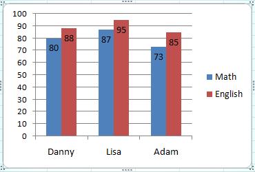
Adding data labels to see the value of the bars in an Excel chart
Multiple Series in One Excel Chart - Peltier Tech Select Series Data: Right click the chart and choose Select Data from the pop-up menu, or click Select Data on the ribbon. As before, click Add, and the Edit Series dialog pops up. There are spaces for series name and Y values. Fill in entries for series name and Y values, and the chart shows two series.
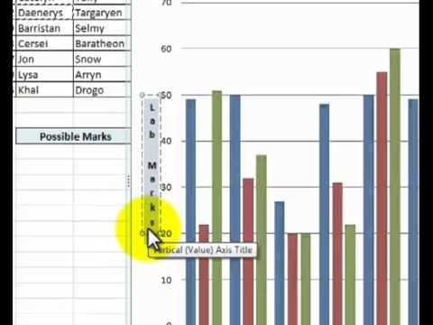
Charts a Chart in Excel: Video 3 - Adding axis labels and changing data formatting - YouTube
excel - Change format of all data labels of a single series at once ... According to this, Workaround 1: Fill up all empty cells referred to. Change the format of labels. Remove added contents. Workaround 2: Change to a dummy range for the data labels, which has no empty cells. Change the format of labels. Switch back to your intended range.
![Asset Allocation Chart Turns Zombie [ChartBusters #1] | Chandoo.org - Learn Microsoft Excel Online](http://assets.chandoo.org/img/cb/asset-allocation-chart-option4.png)
Asset Allocation Chart Turns Zombie [ChartBusters #1] | Chandoo.org - Learn Microsoft Excel Online
How to Change Excel Chart Data Labels to Custom Values? May 05, 2010 · First add data labels to the chart (Layout Ribbon > Data Labels) Define the new data label values in a bunch of cells, like this: Now, click on any data label. This will select “all” data labels. Now click once again. At this point excel will select only one data label.
Create a Histogram Graph in Excel
peltiertech.com › prevent-overlapping-data-labelsPrevent Overlapping Data Labels in Excel Charts - Peltier Tech May 24, 2021 · I recently wrote a post called Slope Chart with Data Labels which provided a simple VBA procedure to add data labels to a slope chart; the procedure simplified the problem caused by positioning each data label individually for each point in the chart. The problem is that often points are located close to each other; the result: overlapping data ...
November 2018
45 excel graph data labels different series This method will introduce a solution to add all data labels from a different column in an Excel chart at the same time. Please do as follows: 1. Right click the data series in the chart, and select Add Data Labels > Add Data Labels from the context menu to add data labels. 2. Right click the data series, and select Format Data Labels from the ...
Add a label and other information to axes in a Graph or Chart in Excel by Excel Made Easy
Understanding Excel Chart Data Series, Data Points, and Data Labels Select a data series in a column chart. All columns of the same color are highlighted. Each column is surrounded by a border that includes small dots on the corners. Select the column in the chart to be modified. Only that column is highlighted. Select the Format tab.

31 How To Label Graphs In Excel - Labels Design Ideas 2020
Prevent Overlapping Data Labels in Excel Charts - Peltier Tech May 24, 2021 · Overlapping Data Labels. Data labels are terribly tedious to apply to slope charts, since these labels have to be positioned to the left of the first point and to the right of the last point of each series. This means the labels have to be tediously selected one by one, even to apply “standard” alignments.
How to Data Labels in a Bar Graph in Excel 2010 - YouTube
engineerexcel.com › 3-axis-graph-excel3 Axis Graph Excel Method: Add a Third Y-Axis - EngineerExcel Next, I added a fourth data series to create the 3 axis graph in Excel. The x-values for the series were the array of constants and the y-values were the unscaled values. I also modified the line style to match the weight of the other gridlines, added markers (the kind that look like plus signs), and changed the color of the line and marker to ...
Programmatically adding excel data labels in a bar chart | ProgressTalk.com
Data labels using values from different series Format the data labels to show the way you want (PHD has some great tips on chart label formatting) Set the third series name to "" and the fill to No Fill and the border to No Line. Depending on your chart type you may need to put the third series on the second axis to get alignment correct. Register To Reply 06-07-2009, 07:22 AM #3 Andy Pope
Post a Comment for "38 excel graph data labels different series"